Figures

On this page you can find all figures and code to produce the figures of the manuscript.

Introduction

Figure 1

#%% Load packages & set directories
import os, sys, pickle
import numpy as np
import matplotlib.pyplot as plt
from scipy import signal
from pathlib import Path

# Set directories
cwd = Path.cwd()
baseDir = cwd.parent
dataDir = baseDir / 'data'
funcDir = baseDir / 'analysis' / 'functions'
sys.path.append(str(funcDir))

import cust_fig, hillmodel

plt.close('all')

#%% Load muscle parameters
mus = 'GMe3'
parFile = os.path.join(dataDir,mus,mus+'_IM.pkl')
muspar = pickle.load(open(parFile, 'rb'))[0]
eseerelmax = (muspar['fmax']/muspar['ksee'])**0.5/muspar['lsee0']
lmtcOpt = muspar['lce_opt']+(1+eseerelmax)*muspar['lsee0']
lmtc0 = lmtcOpt+0.5e-3 # [m] MTC-length at t=0

#%% Generate SIN data
cf = 4
amp = 2*1e-3
   
time = np.linspace(0,5/cf,1000)
lmtc = np.cos(time*2*np.pi*cf)*amp+lmtc0

# Simlation to obtain fsee(t)
gamma0 = muspar['gamma_0']
lcerel0 = hillmodel.force_eq(lmtc[0],gamma0,muspar)[1]
c_in = {}
c_in['time'] = time
c_in['lmtc'] = lmtc
c_in['t_stim'] = np.array([[0, 0.3/cf], [1/cf, 1.3/cf], [2/cf, 2.3/cf], [3/cf, 3.3/cf], [4/cf, 4.3/cf]])

solstr = hillmodel.solve_simu_mtc(gamma0,lcerel0,muspar,c_in)[1]
time, lmtc, stim, gamma, lcerel, q, lsee, lpee, fisomrel, fsee, fpee, fce, fcerel, vcerel = solstr

#%%
cust_fig.style(plt, fontname='Minion Pro',fontsize=11,grid='on')

fig = plt.figure(figsize=(15.92/2.54+0.084, (3.34)/2.54), constrained_layout=True)
gs = fig.add_gridspec(1,3)
axs = np.array([[fig.add_subplot(gs[i, j]) for j in range(gs.ncols)] for i in range(gs.nrows)])

iStart = np.argmin(abs(time-4/cf))
iStop = np.argmin(abs(time-5/cf))
time = time[iStart:iStop]-time[iStart]
lmtc = lmtc[iStart:iStop]
fsee = fsee[iStart:iStop]+2
iPeak = signal.find_peaks(-lmtc,distance=200)[0][0]

# W+
lmtcPos = np.hstack((lmtc[0], lmtc[:iPeak], lmtc[iPeak]))
fseePos = np.hstack((0, fsee[:iPeak], 0))
axs[0,0].plot(lmtc[:iPeak],fsee[:iPeak],'k')
axs[0,0].fill(lmtcPos,fseePos,'#bfbfbf')

# W-
lmtcNeg = np.hstack((lmtc[iPeak], lmtc[iPeak:], lmtc[-1]))
fseeNeg = np.hstack((0, fsee[iPeak:], 0))
axs[0,1].plot(lmtc[iPeak:],fsee[iPeak:],'k')
axs[0,1].fill(lmtcNeg,fseeNeg,'#bfbfbf')

# Wnet
axs[0,2].plot(lmtc,fsee,'k')
axs[0,2].fill(lmtc,fsee,'#bfbfbf')

# Text
axs[0,0].text(np.median(lmtc),fsee[50]/2,'Positive work',ha='center',va='center',)
axs[0,1].text(np.median(lmtc),fsee[150]/2-0.21,'Negative work',ha='center',va='center',)
axs[0,2].text(np.median(lmtc),fsee[50]+(fsee[150]-fsee[50])/2,'Net work',ha='center',va='center',)

# Labels
axs[0,0].set_xlabel('MTC length')
axs[0,1].set_xlabel('MTC length')
axs[0,2].set_xlabel('MTC length')
axs[0,0].set_ylabel('MTC force')
# axs[0,1].set_ylabel('Muscle force')
# axs[0,2].set_ylabel('Muscle force')

# Limits & ticks
axs[0,0].set_xticks([])
axs[0,1].set_xticks([])
axs[0,2].set_xticks([])

axs[0,0].set_yticks([0])
axs[0,1].set_yticks([0])
axs[0,2].set_yticks([0])

axs[0,0].tick_params(direction='out', length=0)
axs[0,1].tick_params(direction='out', length=0)
axs[0,2].tick_params(direction='out', length=0)

axs[0,0].set_xlim(lmtc.min()-0.0003,lmtc.max()+0.0003)
axs[0,1].set_xlim(lmtc.min()-0.0003,lmtc.max()+0.0003)
axs[0,2].set_xlim(lmtc.min()-0.0003,lmtc.max()+0.0003)

axs[0,0].set_ylim(0,10)
axs[0,1].set_ylim(0,10)
axs[0,2].set_ylim(0,10)

# x1, x2 = lmtc[60], lmtc[40]
# y1, y2 = fsee[60]+1, fsee[40]+1
# axs[0].annotate("", xy=(x1, y1), xytext=(x2, y2),arrowprops=dict(arrowstyle="->"))

# x1, x2 = lmtc[140], lmtc[160]
# y1, y2 = fsee[140]+1, fsee[160]+1
# axs[1].annotate("", xy=(x1, y1), xytext=(x2, y2),arrowprops=dict(arrowstyle="<-"))

for i in [25, 50, 75]:
    x1, x2 = lmtc[i], lmtc[i+1]
    y1, y2 = fsee[i], fsee[i+1]
    axs[0,0].annotate("", xy=(x1, y1), xytext=(x2, y2),arrowprops=dict(arrowstyle="<-"))

for i in [125, 150, 175]:
    x1, x2 = lmtc[i], lmtc[i+1]
    y1, y2 = fsee[i], fsee[i+1]
    axs[0,1].annotate("", xy=(x1, y1), xytext=(x2, y2),arrowprops=dict(arrowstyle="<-"))

for i in [25,50,75, 125,150,175]:
    x1, x2 = lmtc[i], lmtc[i+1]
    y1, y2 = fsee[i], fsee[i+1]
    axs[0,2].annotate("", xy=(x1, y1), xytext=(x2, y2),arrowprops=dict(arrowstyle="<-"))


# Add the '-' sign between Plot 1 and Plot 2
# axs[0].text(1.1, 0.5, '–', fontsize=30, va='center', ha='center', transform=axs[0].transAxes, weight='bold')

# Add the '=' sign between Plot 2 and Plot 3
# axs[1].text(1.1, 0.5, '=', fontsize=30, va='center', ha='center', transform=axs[1].transAxes)

labels = ['A','B','C']
cust_fig.add_labels(fig, axs.flatten(), labels)

# %% Show and save
plt.show()
# fig.savefig("i_workloop.png", bbox_inches="tight", pad_inches=0, dpi=600)
fig.savefig("i_workloop.pdf", bbox_inches="tight", pad_inches=0)
# fig.savefig("i_workloop.svg", bbox_inches="tight", pad_inches=0)

# %% Checks
if len(sys.argv) > 1:
    check_size = sys.argv[1]
else:
    check_size = True  

if check_size == True or check_size == 'True':
    cust_fig.report_axes_size(fig,axs)
    # cust_fig.report_fig_size("i_workloop.png") 
    cust_fig.report_fig_size("i_workloop.pdf") 
    # cust_fig.report_fig_size("i_workloop.svg")

Figure 1: An example of a work loop. In a work loop, MTC force is plotted against MTC length (change). The area enclosed by the work loop represents the net mechanical work produced during a full cycle (C), which is the sum of the positive mechanical work during MTC shortening (A) and the negative mechanical work during MTC lengthening (B). The arrows indicate the direction of the work loop over time.

Figure 2

#%% Load packages & set directories
import sys
import numpy as np
import matplotlib.pyplot as plt
from pathlib import Path

# Set directories
cwd = Path.cwd()
baseDir = cwd.parent
dataDir = baseDir / 'data'
funcDir = baseDir / 'analysis' / 'functions'
sys.path.append(str(funcDir))

import cust_fig, trajectories

plt.close('all')

#%% Generate lmtc(t)
cf = 1
fts = 0.65
amp = 1 # [m]
lmtcAvg = 0
acc = 100

time = np.linspace(0,1/cf,1000)
lmtc = trajectories.scv(time,cf,fts,amp,lmtcAvg,acc)[0]

#%% Make figure
cust_fig.style(plt, fontname='Minion Pro',fontsize=11,grid='on')

fig = plt.figure(figsize=(7.96/2.54+0.002, (4.80)/2.54), constrained_layout=True)
fig.set_constrained_layout_pads(w_pad=0, h_pad=0, hspace=0, wspace=0)
gs = fig.add_gridspec(1,1)
axs = np.array([[fig.add_subplot(gs[i, j]) for j in range(gs.ncols)] for i in range(gs.nrows)])

#%% Plot
ax = axs[0,0]
ax.plot(time,lmtc,'k')
ax.set_xlim(0,1/cf+0.05)
ax.set_ylim(-1.2,1.1)

# Plot amp arrow
ax.annotate("", xy=(0, -1), xytext=(0, 1),
            arrowprops=dict(arrowstyle="<->"))
text = ax.text(-0.075,0, "MTC/muscle fibre \n length excursion", color='k',ha='center', va='center', rotation = 90)

#
ax.annotate("", xy=(fts/cf, -1.1), xytext=(0, -1.1),
            arrowprops=dict(arrowstyle="<->"))
ax.text(fts/cf/2,-1.35, '\large $T_{short}$', color='k',ha='center', usetex=True)

ax.annotate("", xy=(1, -1.1), xytext=(fts/cf, -1.1),
            arrowprops=dict(arrowstyle="<->"))
ax.text(fts/cf+(1-fts)/cf/2,-1.35, "\large $T_{length}$", color='k',ha='center', usetex=True)

# CF & FTS
ax.text(
    -0.128, -1.8,
    #r"$\substack{\text{\normalsize Cycle} \\ \text{\normalsize frequency}} = \frac{1}{T_{short} + T_{length}}$",
    r"\large $\substack{\text{Cycle} \\ \text{frequency}} \ = \ $" +r"\Large $\frac{1}{T_{short} + T_{length}}$",
    color='k',
    ha='left',
    va='center',
    usetex=True
)
ax.text(
    1/cf,-1.8,
    #r"$\text{\normalsize FTS} = \frac{T_{short}}{T_{short} + T_{length}}$",
    r"\normalsize $\text{FTS} \ = \ $" + r"\Large $\frac{T_{short}}{T_{short} + T_{length}}$",
    color='k',
    ha='right',
    va='center',
    usetex=True
)

ax.set_xticks([0,fts/cf,1/cf])
ax.set_xticklabels(['','','']) 
ax.set_yticks([])
# ax.set_yticks([-1,0,1])
# ax.set_yticklabels(['','$L_{MTC}^{avg}$',''])
# ax.set_yticklabels(['$L_{MTC}^{avg} - AMP$','$L_{MTC}^{avg}$','$L_{MTC}^{avg} + AMP$']) 
ax.spines['bottom'].set_visible(False)
ax.spines['left'].set_visible(False)

# %% Show and save
plt.show()
# fig.savefig("i_ssc_parameterisation.png", bbox_inches="tight", pad_inches=0, dpi=600)
fig.savefig("i_ssc_parameterisation.pdf", bbox_inches="tight", pad_inches=0)
# fig.savefig("i_ssc_parameterisation.svg", bbox_inches="tight", pad_inches=0)

# %% Checks
if len(sys.argv) > 1:
    check_size = sys.argv[1]
else:
    check_size = True  

if check_size == True or check_size == 'True':
    cust_fig.report_axes_size(fig,axs)
    # cust_fig.report_fig_size("i_ssc_parameterisation.png") 
    cust_fig.report_fig_size("i_ssc_parameterisation.pdf") 
    # cust_fig.report_fig_size("i_ssc_parameterisation.svg") 

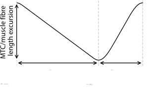
Figure 2: Representation of the parameterisation of stretch-shortening cycles. \(T_{short}\) and \(T_{leng}\) denote the shortening and lengthening durations, respectively, of either the muscle-tendon-complex (MTC) or the muscle fibres. FTS denotes the fraction of the cycle time spent shortening. In the example shown, the MTC/muscle fibres shorten 65% of the cycle duration (i.e., FTS = 0.65).

Methods

Figure 3

# %%
from PIL import Image
import matplotlib.pyplot as plt

# %%
# Load PNG
img = Image.open("m_setup.png")

# Display
plt.imshow(img)
plt.axis("off")
plt.show()

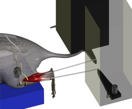
Figure 3: Representation of the experimental setup that provided full control of MTC length and stimulation while measuring m. gastrocnemius medialis (GM) force. GM was carefully exposed from its surrounding tissue and positioned in the setup such that GM pulled in its natural direction, while the femur and foot were securely fixated. The distal end of the calcaneal tendon was connected to a motor via a steel rod. The distal tendon of m. gastrocnemius lateralis and m. plantaris was connected to a second motor. A cuff-electrode was placed on n. ischiadicus. N. peroneus, n. suralis and the branch of n. ischiadicus innervating m. gastrocnemius lateralis and m. soleus were cut such that only GM was innervated.

Figure 4

#%% Load packages & set directories
import sys
import numpy as np
import matplotlib.pyplot as plt
from pathlib import Path

# Set directories
cwd = Path.cwd()
baseDir = cwd.parent
dataDir = baseDir / 'data'
funcDir = baseDir / 'analysis' / 'functions'
sys.path.append(str(funcDir))

import cust_fig
plt.close('all')

#%%
cust_fig.style(plt, fontname='Minion Pro',fontsize=11,grid=False)

fig = plt.figure(figsize=(15.92/2/2.54+0.084, (15.92/2+1.74)/2.54), constrained_layout=True)
gs = fig.add_gridspec(1, 1)
axs = np.array([[fig.add_subplot(gs[i, j]) for j in range(gs.ncols)] for i in range(gs.nrows)])
ax = axs[0,0]

#%%    
cfCondA  = [1,2,3,4,5,3,3,3,3,5,4,2,1]
cfCondB  = [1,1.5,2,2.5,3,2,2,2,2,3,2.5,1.5,1]
ftsCond = [0.5, 0.5, 0.5, 0.5, 0.5, 0.8, 0.65, 0.35, 0.20, 0.80, 0.65, 0.35, 0.20]

for idx,(cfA,cfB,fts) in enumerate(zip(cfCondA,cfCondB,ftsCond)):
    ax.text(cfA, fts, str(idx+1), bbox=dict(facecolor='white',boxstyle='circle'),ha='center',va='center')
    ax.text(1, 0.5, "1", bbox=dict(facecolor='white',boxstyle='circle'),ha='center',va='center')
    ax.text(2, 0.5, "2", bbox=dict(facecolor='white',boxstyle='circle'),ha='center',va='center')
    ax.text(3, 0.5, "3", bbox=dict(facecolor='white',boxstyle='circle'),ha='center',va='center')
    ax.text(4, 0.5, "4", bbox=dict(facecolor='white',boxstyle='circle'),ha='center',va='center')
    ax.text(5, 0.5, "5", bbox=dict(facecolor='white',boxstyle='circle'),ha='center',va='center')
    ax.text(3, 0.8, "6", bbox=dict(facecolor='white',boxstyle='circle'),ha='center',va='center')
    ax.text(3, 0.65, "7", bbox=dict(facecolor='white',boxstyle='circle'),ha='center',va='center')
    ax.text(3, 0.35, "8", bbox=dict(facecolor='white',boxstyle='circle'),ha='center',va='center')
    ax.text(3, 0.2, "9", bbox=dict(facecolor='white',boxstyle='circle'),ha='center',va='center')
    ax.text(5, 0.8, "10", bbox=dict(facecolor='white',boxstyle='circle'),ha='center',va='center')
    ax.text(4, 0.65, "11", bbox=dict(facecolor='white',boxstyle='circle'),ha='center',va='center')
    ax.text(2, 0.35, "12", bbox=dict(facecolor='white',boxstyle='circle'),ha='center',va='center')
    ax.text(1, 0.2, "13", bbox=dict(facecolor='white',boxstyle='circle'),ha='center',va='center')
 
ax.set_ylabel('FTS [ ]')
ax.set_xlabel('Cycle frequency [Hz] \n SSCs with 4 mm MTC length excursion')

ax.set_xlim(0.5,5.5)
ax.set_xticks([1,2,3,4,5])
ax.set_ylim(0.1,0.9)
ax.set_yticks([0.2,0.35,0.5,0.65,0.8])

axB = ax.twiny()
ax = axB
ax.set_xlim(0.5,5.5)
ax.set_xticks([1,2,3,4,5])
ax.set_xticklabels(['1','1.5','2','2.5','3'])
ax.set_xlabel('Cycle frequency [Hz] \n SSCs with 8 mm MTC length excursion')
ax.spines['top'].set_visible(True)

# labels = ['A','B']
# cust_fig.add_labels(fig, axs.flatten(), labels)

# %% Show and save
plt.show()
# fig.savefig("m_conditions.png", bbox_inches="tight", pad_inches=0, dpi=600)
fig.savefig("m_conditions.pdf", bbox_inches="tight", pad_inches=0)
# fig.savefig("m_conditions.svg", bbox_inches="tight", pad_inches=0)

# %% Checks
if len(sys.argv) > 1:
    check_size = sys.argv[1]
else:
    check_size = True  

if check_size == True or check_size == 'True':
    cust_fig.report_axes_size(fig,axs)
    # cust_fig.report_fig_size("m_conditions.png") 
    cust_fig.report_fig_size("m_conditions.pdf") 
    # cust_fig.report_fig_size("m_conditions.svg")

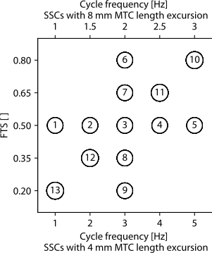
Figure 4: Representation of experimentally investigated SSCs. Thirteen combinations of cycle frequency and FTS were tested at two distinct MTC length excursions (4 mm and 8 mm), resulting in a total of 26 experimental SSC conditions.

Results

Figure 5

#%% Load packages & set directories
import os, sys
import pandas as pd
import numpy as np
import matplotlib.pyplot as plt
from pathlib import Path

# Set directories
cwd = Path.cwd()
baseDir = cwd.parent
dataDir = baseDir / 'data'
funcDir = baseDir / 'analysis' / 'functions'
sys.path.append(str(funcDir))

import cust_fig

plt.close('all')

#%%
cust_fig.style(plt, fontname='Minion Pro',fontsize=11,grid=False)

fig = plt.figure(figsize=(15.92/2.54+0.001, 10.32/2.54), constrained_layout=True)
fig.set_constrained_layout_pads(w_pad=0, h_pad=0, hspace=0, wspace=0)
gs = fig.add_gridspec(2,2)
axs = [fig.add_subplot(gs[i]) for i in range(0,gs.ncols*gs.nrows)]

#%%
colorSet = plt.rcParams['axes.prop_cycle'].by_key()['color']
colorSet[0] = '#000000'

lines = []
for iMus,(mus,clr) in enumerate(zip(['GMe1','GMe2','GMe3'],colorSet)):
    dataDirMus = os.path.join(dataDir,mus,'')
    dataExp = pd.read_excel(dataDirMus+str(mus)+'_dataAMPO.xlsx').to_numpy()[:,5:].astype(float)
    
    dataExp[dataExp<1] = np.nan
    dataSSC_PA_T1 = np.nanmean(dataExp[0:3,:],axis=0)
    dataSSC_PA_T2 = np.nanmean(dataExp[3:6,:],axis=0)
    dataSSC_PB_T1 = np.nanmean(dataExp[6:9,:],axis=0)
    dataSSC_PB_T2 = np.nanmean(dataExp[9:12,:],axis=0)
        
    for iExp,exp in enumerate(['SSC_PA', 'SSC_PB']):
        if exp == 'SSC_PA': # 2mm amplitude
            iRow = np.r_[0,1,2]
            
            # CF
            iCol = np.r_[1,2,3,4,5]-1
            # Trial 1
            AMPO = dataSSC_PA_T1[iCol]
            axs[iExp].scatter([1,2,3,4,5],AMPO,color=clr, marker='x',s=20, clip_on=False)
            AMPO = dataSSC_PA_T2[iCol]
            axs[iExp].scatter([1,2,3,4,5],AMPO,color=clr, marker='.',s=40, clip_on=False)
            
            # FTS
            iCol = np.r_[6,7,5,8,9]-1 
            # Trial 1
            AMPO = dataSSC_PA_T1[iCol]
            axs[iExp+2].scatter([0.8,0.65,0.50,0.35,0.20],AMPO,color=clr, marker='x',s=20, clip_on=False)
            # Trial 2
            AMPO = dataSSC_PA_T2[iCol]
            axs[iExp+2].scatter([0.8,0.65,0.50,0.35,0.20],AMPO,color=clr, marker='.',s=40, clip_on=False)
            
        elif exp == 'SSC_PB': # 4mm amplitude
            iRow = np.r_[6,7,8] 
            
            # CF
            iCol = np.r_[1,2,3,4,5]-1
            # Trial 1
            AMPO = dataSSC_PB_T1[iCol]
            l1 = axs[iExp].scatter([1.0,1.5,2.0,2.5,3.0],AMPO,color=clr, marker='x',s=20, clip_on=False)
            AMPO = dataSSC_PB_T2[iCol]
            l2 = axs[iExp].scatter([1.0,1.5,2.0,2.5,3.0],AMPO,color=clr, marker='.',s=40, clip_on=False)
            lines.append(l1)
            
            if iMus == 0:
                l = [l1, l2]
            
            # FTS
            iCol = np.r_[6,7,5,8,9]-1 
            # Trial 1
            AMPO = dataSSC_PB_T1[iCol]
            axs[iExp+2].scatter([0.8,0.65,0.50,0.35,0.20],AMPO,color=clr, marker='x',s=20, clip_on=False)
            # Trial 2
            AMPO = dataSSC_PB_T2[iCol]
            axs[iExp+2].scatter([0.8,0.65,0.50,0.35,0.20],AMPO,color=clr, marker='.',s=40, clip_on=False)
        
legend = axs[1].legend(lines,
                       ['1', '2', '3'],
                       loc='lower right',
                       title='Rat',
                       title_fontproperties={'weight': 'bold'},
                       alignment='right')
legend = axs[3].legend(l,
                       ['1', '2'],
                       loc='lower right',
                       title='Trial',
                       title_fontproperties={'weight': 'bold'},
                       alignment='right')

# #%% Plot
axs[0].set_xlabel('Cycle frequency [Hz]')
axs[1].set_xlabel('Cycle frequency [Hz]')
axs[2].set_xlabel('FTS [ ]')
axs[3].set_xlabel('FTS [ ]')
axs[0].set_ylabel('AMPO [mW]')
axs[2].set_ylabel('AMPO [mW]')

# Subplot 0,0: Imposed CF - 4mm MLE
ax = axs[0]
ax.set_xlim(1,5)
ax.set_xticks([1,2,3,4,5])
# ax.set_ylim(0,97.5)
# ax.set_yticks([0,30,60,90])
# ax.set_yticks([15,45,75], minor=True)
ax.set_ylim(0,130)
ax.set_yticks([0,40,80,120])
ax.set_yticks([20,60,100], minor=True)

# Subplot 0,1: Iposed CF - 8mm MLE
ax = axs[1]
ax.set_xlim(1,3)
ax.set_xticks([1,1.5,2,2.5,3])
# ax.set_ylim(0,97.5)
# ax.set_yticks([0,30,60,90])
# ax.set_yticks([15,45,75], minor=True)
ax.set_ylim(0,130)
ax.set_yticks([0,40,80,120])
ax.set_yticks([20,60,100], minor=True)

# Subplot 1,0: Imposed FTS - 4mm MLE
ax = axs[2]
ax.set_xlim(0.2,0.8)
ax.set_xticks([0.2,0.35,0.5,0.65,0.8])
ax.set_ylim(0,130)
ax.set_yticks([0,40,80,120])
ax.set_yticks([20,60,100], minor=True)

# Subplot 1,1: Imposed FTS - 8mm MLE
ax = axs[3]
ax.set_xlim(0.2,0.8)
ax.set_xticks([0.2,0.35,0.5,0.65,0.8])
ax.set_ylim(0,130)
ax.set_yticks([0,40,80,120])
ax.set_yticks([20,60,100], minor=True)

#%%
for ax in [axs[0], axs[1], axs[2], axs[3]]:
    ax.spines['left'].set_position(('outward', 12))
    
fig.align_ylabels(axs)
cust_fig.add_labels(fig,axs,['A','B','C', 'D'],-15/72)

# %% Show and save
plt.show()
# fig.savefig("r_ampo_cf_fts.png", bbox_inches="tight", pad_inches=0, dpi=600)
fig.savefig("r_ampo_cf_fts.pdf", bbox_inches="tight", pad_inches=0)
# fig.savefig("r_ampo_cf_fts.svg", bbox_inches="tight", pad_inches=0)

# %% Checks
if len(sys.argv) > 1:
    check_size = sys.argv[1]
else:
    check_size = True  

if check_size == True or check_size == 'True':
    cust_fig.report_axes_size(fig,axs)
    # cust_fig.report_fig_size("r_ampo_cf_fts.png") 
    cust_fig.report_fig_size("r_ampo_cf_fts.pdf") 
    # cust_fig.report_fig_size("r_ampo_cf_fts.svg")

<positron-console-cell-9>:47: RuntimeWarning: Mean of empty slice

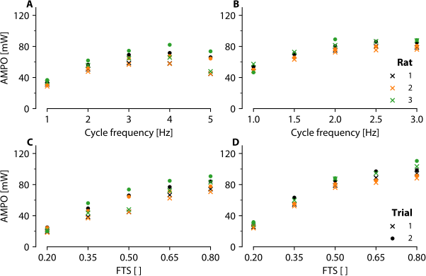
Figure 5: Experimentally measured influence of cycle frequency and FTS on AMPO. AMPO as a function of cycle frequency, with a fixed FTS of 0.5 at an MTC length excursion of 4 mm (A) and 8 mm (B). AMPO as a function of FTS, with a fixed cycle frequency of 3 Hz at an MTC length excursion of 4 mm (C) and 8 mm (D). Each combination of cycle frequency, FTS and MTC length excursion was performed twice. The first trial with suboptimal muscle stimulation duration and the second trial with an improved muscle stimulation duration.

Figure 6

#%% Load packages & set directories
import os, glob, sys, pickle
import pandas as pd
import matplotlib.pyplot as plt
from scipy import signal
from pathlib import Path

# Set directories
cwd = Path.cwd()
baseDir = cwd.parent
dataDir = baseDir / 'data'
funcDir = baseDir / 'analysis' / 'functions'
sys.path.append(str(funcDir))

import cust_fig, stimulation

plt.close('all')

#%% Select rat
mus = 'GMe1'
parFile = os.path.join(dataDir,mus,mus+'_IM.pkl')
muspar = pickle.load(open(parFile, 'rb'))[0]

#%%
cust_fig.style(plt, fontname='Minion Pro',fontsize=11,grid=False)
fig = plt.figure(figsize=(15.92/2.54+51/600, 10.9/2.54), constrained_layout=True) # 3:2 ratio
gs = fig.add_gridspec(4, 2, height_ratios=[5.0,1,35,35],wspace=0.1)
axs = [fig.add_subplot(gs[i]) for i in range(0,gs.ncols*gs.nrows)]

colorSet = plt.rcParams['axes.prop_cycle'].by_key()['color']
colorSet[0] = '#000000'

#%% SSC: CF = 3 Hz, FTS = 0.5 Hz, MLE = 4mm
iCond = 5
fileExp = sorted(glob.glob(os.path.join(dataDir,mus,'dataExp','SSC_PA','*.csv')))[iCond]
fileSim = sorted(glob.glob(os.path.join(dataDir,mus,'simsExp','SSC_PA','*.csv')))[iCond]

if fileExp[-19:-4] != fileSim[-22:-7]:
    print(fileExp[-19:-4])
    print(fileSim[-22:-7])
    print('Datafile and simulation not the same!')
    sys.exit()
if fileExp[-19:-4] != 'GMe1_SSC_PA03_2': 
    print('Wrong files loaded..')
    sys.exit()

# Experimental data
df = pd.read_csv(fileExp)
data = df.to_numpy()
time,lmtc,stim,fsee = data.T[0:4]

iMin = signal.find_peaks(-lmtc[150:],distance=200)[0]+150
iMax = signal.find_peaks(lmtc[150:],distance=200)[0]+150
iSel = slice(iMin[0],iMax[3])
tOff = time[iMin[0]]
time = time[iSel]-tOff
lmtc = lmtc[iSel]
fsee = fsee[iSel]
stim = stim[iSel]

axs[0].plot(time,lmtc*1e3, color=colorSet[0])
axs[4].plot(time,fsee, color=colorSet[0])
axs[6].plot(lmtc*1e3,fsee, color=colorSet[0])

# Simulated data
df = pd.read_csv(fileSim)
data = df.to_numpy()
time,lmtc,stim,fsee = data.T[0:4]

tOff = time[iMin[0]]
time = time[iSel]-tOff
lmtc = lmtc[iSel]
fsee = fsee[iSel]
stim = stim[iSel]

# axs[0].plot(time,lmtc*1e3,'--', color=colorSet[1])
axs[4].plot(time,fsee,'--', color=colorSet[1])
axs[6].plot(lmtc*1e3,fsee, '--', color=colorSet[1])

tStimOn, tStimOff = stimulation.get_stim_timing(time,stim)
cust_fig.plot_stim(axs[2],tStimOn[0],tStimOff[0],y=0, lw=1/3)
cust_fig.plot_stim(axs[2],tStimOn[1],tStimOff[1],y=0, lw=1/3)
cust_fig.plot_stim(axs[2],tStimOn[2],tStimOff[2],y=0, lw=1/3)

for ax in [axs[0], axs[2], axs[4]]:
    ax.set_xlim(time[0],time[-1])

#%% SSC: CF = 2 Hz, FTS = 0.5 Hz, MLE = 8mm
iCond = 6
fileExp = sorted(glob.glob(os.path.join(dataDir,mus,'dataExp','SSC_PB','*.csv')))[iCond]
fileSim = sorted(glob.glob(os.path.join(dataDir,mus,'simsExp','SSC_PB','*.csv')))[iCond]

if fileExp[-19:-4] != fileSim[-22:-7]:
    print(fileExp[-19:-4])
    print(fileSim[-22:-7])
    print('Datafile and simulation not the same!')
    sys.exit()
if fileExp[-19:-4] != 'GMe1_SSC_PB03_2': 
    print('Wrong files loaded..')
    sys.exit()

# Experimental data
df = pd.read_csv(fileExp)
data = df.to_numpy()
time,lmtc,stim,fsee = data.T[0:4]

iMin = signal.find_peaks(-lmtc[150:],distance=200)[0]+150
iMax = signal.find_peaks(lmtc[150:],distance=200)[0]+150
iSel = slice(iMin[0],iMax[3])
tOff = time[iMin[0]]
time = time[iSel]-tOff
lmtc = lmtc[iSel]
fsee = fsee[iSel]
stim = stim[iSel]

axs[1].plot(time,lmtc*1e3, color=colorSet[0])
l1, = axs[5].plot(time,fsee, color=colorSet[0], label='Measured')
axs[7].plot(lmtc*1e3,fsee, color=colorSet[0])

# Simulated data
df = pd.read_csv(fileSim)
data = df.to_numpy()
time,lmtc,stim,fsee = data.T[0:4]

tOff = time[iMin[0]]
time = time[iSel]-tOff
lmtc = lmtc[iSel]
fsee = fsee[iSel]
stim = stim[iSel]

# axs[1].plot(time,lmtc*1e3,'--', color=colorSet[1])
l2, = axs[5].plot(time,fsee,'--', color=colorSet[1], label='Predicted')
axs[7].plot(lmtc*1e3,fsee,'--', color=colorSet[1])

tStimOn, tStimOff = stimulation.get_stim_timing(time,stim)
cust_fig.plot_stim(axs[3],tStimOn[0],tStimOff[0],y=0, lw=1/3)
cust_fig.plot_stim(axs[3],tStimOn[1],tStimOff[1],y=0, lw=1/3)
cust_fig.plot_stim(axs[3],tStimOn[2],tStimOff[2],y=0, lw=1/3)

for ax in [axs[1], axs[3], axs[5]]:
    ax.set_xlim(time[0],time[-1])

axs[5].legend(['Measured', 'Predicted'],
    loc='center',
    bbox_to_anchor=(0.525, 0.5),  # shift left (into space between axes) and center vertically
    bbox_transform=fig.transFigure,
    handlelength=0.8,
    handletextpad=0.5,
    labelspacing=0.2,
)

#%% Labels etc.
# Lmtc(t) - SSC_PA
ax = axs[0]
ax.set_ylim(axs[1].get_ylim())
ax.spines['top'].set_visible(False)
ax.spines['right'].set_visible(False)
ax.spines['bottom'].set_visible(False)
ax.spines['left'].set_visible(False)
ax.set_xticks([])
ax.set_yticks([])
y_min, y_max = 41.5, 45.5
ax.set_ylim(y_min, y_max)
y_range = (y_max-y_min)
ax.plot([0, 0], [y_min, y_max], color='black', lw=1)
ax.set_yticks([(y_min+y_max)/2])
ax.set_yticklabels([f'{y_range:.1f} mm'])
ax.tick_params(
    axis='both',       # both x and y axes
    which='both',      # both major and minor ticks
    bottom=False,      # remove ticks on bottom
    top=False,         # remove ticks on top
    left=False,        # remove ticks on left
    right=False        # remove ticks on right
)

# Lmtc(t) - SSC_PB
ax = axs[1]
ax.spines['top'].set_visible(False)
ax.spines['right'].set_visible(False)
ax.spines['bottom'].set_visible(False)
ax.spines['left'].set_visible(False)
ax.set_xticks([])
ax.set_yticks([])
y_min, y_max = 39.5, 47.5
ax.set_ylim(y_min, y_max)
y_range = (y_max-y_min)
ax.plot([0, 0], [y_min, y_max], color='black', lw=1)
ax.set_yticks([(y_min+y_max)/2])
ax.set_yticklabels([f'{y_range:.1f} mm'])
ax.tick_params(
    axis='both',       # both x and y axes
    which='both',      # both major and minor ticks
    bottom=False,      # remove ticks on bottom
    top=False,         # remove ticks on top
    left=False,        # remove ticks on left
    right=False        # remove ticks on right
)



# STIM(t) - SSC_PA
ax = axs[2]
ax.set_ylim(-0.5,0.5)
ax.spines['top'].set_visible(False)
ax.spines['right'].set_visible(False)
ax.spines['bottom'].set_visible(False)
ax.spines['left'].set_visible(False)
ax.set_xticks([])
ax.set_yticks([])

# STIM(t) - SSC_PB
ax = axs[3]
ax.set_ylim(-0.5,0.5)
ax.spines['top'].set_visible(False)
ax.spines['right'].set_visible(False)
ax.spines['bottom'].set_visible(False)
ax.spines['left'].set_visible(False)
ax.set_xticks([])
ax.set_yticks([])

# Fsee(t) - SSC_PA
ax = axs[4]
ax.set_xticks([0,0.4,0.8])
ax.set_xticks([0.2,0.6,1.0],minor=True)
ax.set_ylim(0,9.5)
ax.set_yticks([0,4,8])
ax.set_yticks([2,6],minor=True)
ax.set_ylabel('SEE force [N]')

# Fsee(t) - SSC_PB
ax = axs[5]
ax.set_xticks([0,0.5,1.0,1.5])
ax.set_xticks([0.25,0.75,1.25],minor=True)
ax.set_ylim(0,9.5)
ax.set_yticks([0,4,8])
ax.set_yticks([2,6],minor=True)
# ax.set_ylabel('$F_{SEE}$ [N]')

axs[4].set_xlabel('Time [s]')
axs[5].set_xlabel('Time [s]')

# Fsee(Lmtc) - SSC_PA
ax = axs[6]
ax.set_xlim(41.25,45.75)
ax.set_xticks([42,43,44,45])
ax.set_xticks([41.5,42.5,43.5,44.5,45.5],minor=True)
ax.set_xlabel('MTC length [mm]')
ax.set_ylim(0,9.5)
ax.set_yticks([0,4,8])
ax.set_yticks([2,6],minor=True)
ax.set_ylabel('SEE force [N]')

# Fsee(Lmtc) - SSC_PB
ax = axs[7]
ax.set_xlim(39.25,47.5)
ax.set_xticks([40,42,44,46])
ax.set_xticks([41,43,45,47],minor=True)
ax.set_xlabel('MTC length [mm]')
ax.set_ylim(0,9.5)
ax.set_yticks([0,4,8])
ax.set_yticks([2,6],minor=True)

# fig.align_labels()
cust_fig.add_labels(fig, axs, ['A', 'B'])

# %% Show and save
plt.show()
# fig.savefig("r_exp_vs_pred2.png", bbox_inches="tight", pad_inches=0, dpi=600)
fig.savefig("r_exp_vs_pred.pdf", bbox_inches="tight", pad_inches=0)
# fig.savefig("r_exp_vs_pred2.svg", bbox_inches="tight", pad_inches=0)

# %% Checks
if len(sys.argv) > 1:
    check_size = sys.argv[1]
else:
    check_size = True  

if check_size == True or check_size == 'True':
    cust_fig.report_axes_size(fig,axs)
    # cust_fig.report_fig_size("r_exp_vs_pred.png") 
    cust_fig.report_fig_size("r_exp_vs_pred.pdf") 
    # cust_fig.report_fig_size("r_exp_vs_pred.svg")

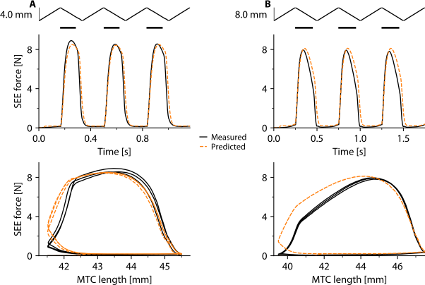
Figure 6: Comparison of experimentally measured and predicted SEE force over time. Predicted SEE force over time was derived using a Hill MTC-type model, with experimentally measured MTC length and stimulation over time as inputs. Predicted SEE force closely matched experimentally measured SEE force during activation but was slightly higher than experimentally measured SEE force during relaxation in most conditions. Top: MTC length over time. Second: Muscle stimulation over time, with maximal stimulation during the periods indicated by the black bars and no stimulation elsewhere. Third: SEE force over time. Bottom: SEE force as a function of MTC length (‘the work loop’). A) SSC with a cycle frequency of 3 Hz, an FTS of 0.5 and an MTC length excursion of 4 mm. B) SSC with a cycle frequency of 2 Hz, an FTS of 0.5 and an MTC length excursion of 8 mm.

Figure 7

#%% Load packages & set directories
import os, sys
import pandas as pd
import numpy as np
import matplotlib.pyplot as plt
from pathlib import Path

# Set directories
cwd = Path.cwd()
baseDir = cwd.parent
dataDir = baseDir / 'data'
funcDir = baseDir / 'analysis' / 'functions'
sys.path.append(str(funcDir))

import cust_fig

plt.close('all')

#%%
cust_fig.style(plt, fontname='Minion Pro',fontsize=11,grid=True)

fig = plt.figure(figsize=(15.92/3/2.54, 5.07/2.54), constrained_layout=True) # 3:2 ratio
fig.set_constrained_layout_pads(w_pad=0, h_pad=0, hspace=0, wspace=0)
gs = fig.add_gridspec(1,1)
axs = [fig.add_subplot(gs[i]) for i in range(0,gs.ncols*gs.nrows)]

colorSet = plt.rcParams['axes.prop_cycle'].by_key()['color']
colorSet[0] = '#000000'
symbols = ['o','^', 's']

#%%
for mus,clr,symbol in zip(['GMe1','GMe2','GMe3'],colorSet,symbols):
    dataDirMus = os.path.join(dataDir,mus,'')
    dataExp = pd.read_excel(dataDirMus+str(mus)+'_dataAMPO.xlsx').to_numpy()[:,5:].astype(float)
    simsExp = pd.read_excel(dataDirMus+str(mus)+'_simsAMPO.xlsx').to_numpy()[:,5:].astype(float)
    
    dataExp[dataExp<1] = np.nan
    simsExp[simsExp<1] = np.nan
        
    axs[0].plot(dataExp.flatten(),simsExp.flatten(),symbol,ms=1,color=clr)

legend = axs[0].legend(['1', '2', '3'],
                       title='Rat',
                       title_fontproperties={'weight': 'bold'},
                       loc='lower right',
                       alignment='right',
                       handlelength=0.8,
                       handletextpad=0.5,
                       labelspacing=0.2)

    
#%% Plot
axs[0].set_xlabel(r'Measured AMPO [mW]')
axs[0].set_ylabel(r'Predicted AMPO [mW]')

axs[0].set_xlim(0,162.5)
axs[0].set_xticks([0,25,50,75,100,125,150])
axs[0].set_xticklabels(['0','','50','','100','','150'])
axs[0].set_ylim(0,162.5)
axs[0].set_yticks([0,25,50,75,100,125,150])
axs[0].set_yticklabels(['0','','50','','100','','150'])

# %% Show and save
plt.show()
# fig.savefig("r_correlation.png", bbox_inches="tight", pad_inches=0, dpi=600)
fig.savefig("r_correlation.pdf", bbox_inches="tight", pad_inches=0)
# fig.savefig("r_correlation.svg", bbox_inches="tight", pad_inches=0)

# %% Checks
if len(sys.argv) > 1:
    check_size = sys.argv[1]
else:
    check_size = True  

if check_size == True or check_size == 'True':
    cust_fig.report_axes_size(fig,axs)
    # cust_fig.report_fig_size("r_correlation.png") 
    cust_fig.report_fig_size("r_correlation.pdf") 
    # cust_fig.report_fig_size("r_correlation.svg")

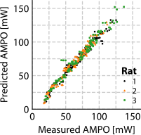
Figure 7: Comparison of experimentally measured and predicted AMPO. Measured AMPO was derived from experimentally observed MTC length and GM force. Predicted AMPO was derived using a Hill MTC-type model, with experimentally measured MTC length and stimulation over time as inputs to predict GM force. Each dot represents AMPO of one full cycle where muscle stimulation was present, such that there are three dots for each experimental SSC condition. The nearly perfect correlation demonstrates that a Hill-type MTC model can accurately predict the influence of MTC length and stimulation over time on AMPO.

Figure 8

#%% Load packages & set directories
import os, sys, pickle
import numpy as np
import pandas as pd
import matplotlib.pyplot as plt
from pathlib import Path

# Set directories
cwd = Path.cwd()
baseDir = cwd.parent
dataDir = baseDir / 'data'
funcDir = baseDir / 'analysis' / 'functions'
sys.path.append(str(funcDir))

import cust_fig, helpers, interpolation, stats

plt.close('all')

#%%
cf_set = np.arange(0.5,6.1,0.5) # [Hz] n = 12
mle_set = np.arange(2,11.1,1)*1e-3 # [m] n = 11

#%%
customlay = cust_fig.style(plt, fontname='Minion Pro',fontsize=11,grid=False)
customlay['xtick.direction'] = 'out' # cause of contour plot
customlay['ytick.direction'] = 'out'
# plt.rcParams.update(plt.rcParamsDefault)
plt.rcParams.update(customlay)

# fig = plt.figure(figsize=(15.92/2.54+0.085, 15.92/2.54+0.363), constrained_layout=True) # 3:2 ratio
fig = plt.figure(figsize=(15.92/2/2.54+51/600, 8.86/2.54), constrained_layout=True) # 3:2 ratio
gs = fig.add_gridspec(2,2)
# axs = [fig.add_subplot(gs[i]) for i in range(0,gs.ncols*gs.nrows)]
axs = [fig.add_subplot(gs[0, 0])]
axs.append(fig.add_subplot(gs[0, 1], sharex=axs[0]))
axs.append(fig.add_subplot(gs[1, 0], sharex=axs[0]))
axs.append(fig.add_subplot(gs[1, 1], sharex=axs[0]))

for iFts, fts in enumerate([0.25, 0.50, 0.75, 0.85]):
    AMPOsets, AMPOfines, sf = [], [], []
    for iMus,mus in enumerate(['GMe1', 'GMe2', 'GMe3']):
        # Load muspar
        parFile = os.path.join(dataDir,mus,mus+'_IM.pkl')
        muspar = pickle.load(open(parFile, 'rb'))[0]
        # sf.append(muspar['lce_opt']*muspar['fmax'])
        sf.append(1)
                
        # Load and interpolate data
        dataDirSim = os.path.join(dataDir,mus,'simsCV','')
        AMPOset = helpers.load_sims(cf_set,fts,mle_set,mus,dataDirSim)
        AMPOfine,(cfFine,mleFine) = interpolation.do_3d(AMPOset,(cf_set,mle_set),N=100,method='cubic')
           
        # Append to list for all muscles
        AMPOset = AMPOset/sf[iMus]
        AMPOsets.append(AMPOset)
        AMPOfine = AMPOfine/sf[iMus]
        AMPOfines.append(AMPOfine)
    
    #%% Calculate average   
    AMPOsets        = np.dstack(AMPOsets)
    AMPOfines       = np.dstack(AMPOfines)
    meanAMPOsets    = np.mean(AMPOsets,2)
    meanAMPOsets    = meanAMPOsets*np.mean(sf)
    meanAMPOfines   = np.mean(AMPOfines,2)
    meanAMPOfines   = meanAMPOfines*np.mean(sf)
    
    #%%
    iRow, iCol = np.unravel_index(np.nanargmax(meanAMPOsets), meanAMPOsets.shape)
    
    # Compute optimum, but interpolate over smaller interval..
    AMPOsets, AMPOfines, sf = [], [], []
    for iMus,mus in enumerate(['GMe1', 'GMe2', 'GMe3']):
        # Load muspar
        parFile = os.path.join(dataDir,mus,mus+'_IM.pkl')
        muspar = pickle.load(open(parFile, 'rb'))[0]
        sf.append(muspar['lce_opt']*muspar['fmax'])
                
        # Load and interpolate data
        dataDirSim = os.path.join(dataDir,mus,'simsCV','')
        AMPOset = helpers.load_sims(cf_set[iRow-1:iRow+2],fts,mle_set[iCol-1:iCol+2],mus,dataDirSim)
        AMPOfine,(cfFine_s,mleFine_s) = interpolation.do_3d(AMPOset,(cf_set[iRow-1:iRow+2],mle_set[iCol-1:iCol+2]),N=100,method='cubic')
           
        # Append to list for all muscles
        AMPOfine = AMPOfine/sf[iMus]
        AMPOfines.append(AMPOfine)
    AMPOfines       = np.dstack(AMPOfines)
    meanAMPOfines_s   = np.mean(AMPOfines,2)
    meanAMPOfines_s = meanAMPOfines_s*np.mean(sf)
    
    AMPOmax, (cfOpt, mleOpt) = stats.find_max(meanAMPOfines_s,(cfFine_s,mleFine_s))
    
    cfOpt2 = 0
    mleOpt2 = 0
    for iMus,mus in enumerate(['GMe1', 'GMe2', 'GMe3']):
        dataDirSim = os.path.join(dataDir,mus,'simsCV','')

        fileName = mus+f'_cfOpt_fts{fts:{"0.2f"}}_mleOpt'
        df = pd.read_csv(dataDirSim+fileName+'.csv')
        data = df.to_numpy()
        time,lmtc,stim,fsee = data.T[0:4]
        cfOpt2 += (1/time[-1])/3
        mleOpt2 += (lmtc.max()-lmtc.min())/3

    # cfOpt = cfOpt2
    # ampOpt = ampOpt2
    
    # print("AMPO = %1.2f mW" % (AMPOmax*1e3))
    # print("CF = %1.2f Hz" % cfOpt)
    # print("MLE = %1.2f mm" % (mleOpt*1e3))
    
    #%% Make figure 
    if fts == 0.50 or fts == 0.75:
        contour_levels  = np.arange(10,AMPOmax*1e3,20)
    else:
        contour_levels  = np.arange(0,AMPOmax*1e3,20)
    
    cmap = plt.get_cmap('gray_r')
    cmap = cust_fig.truncate_colormap(cmap, 0.25, 1)
    
    iAx = iFts
    CS = axs[iAx].contour(cfFine,mleFine*1e3,meanAMPOfines*1e3, contour_levels,cmap=cmap)
    # axs[iAx].plot(cfOpt,ampOpt*1e3*2,'kx',markersize=4)
    axs[iAx].scatter(cfOpt,mleOpt*1e3, marker='^', facecolors='none', edgecolors='k', s=15)
    axs[iAx].text(cfOpt-5.5*0.02,mleOpt*1e3+9*0.02, f'{AMPOmax*1e3:0.0f}', fontsize='x-small', va='bottom', ha='right')
    
    axs[iAx].set_xlim([0.5, axs[iAx].get_xlim()[1]])
    axs[iAx].set_title(f'FTS = {fts:0.2f}')
    
    a = (11-2)/5.5  # Example: y = x
    b = 2-0.5*a
    
    def line_func(x):
        return a * x + b

    # Function to compute intersection between segment and line
    def segment_line_intersection(p1, p2, a, b):
        x1, y1 = p1
        x2, y2 = p2
        # Represent line segment as p + t*r, intersect with line y = ax + b
        denom = (y2 - y1) - a * (x2 - x1)
        if denom == 0:
            return None  # Parallel
        t = ((a * x1 + b) - y1) / denom
        if 0 <= t <= 1:
            x_int = x1 + t * (x2 - x1)
            y_int = y1 + t * (y2 - y1)
            if np.isclose(y_int, a * x_int + b):
                return x_int, y_int
        return None

    # Find intersection points to use for manual labels
    manual_locations = []

    for i, segs in enumerate(CS.allsegs):
        for seg in segs:
            for j in range(len(seg) - 1):
                p1, p2 = seg[j], seg[j + 1]
                pt = segment_line_intersection(p1, p2, a, b)
                if pt is not None:
                    manual_locations.append(pt)
    # if fts == 0.50:
    #     del(manual_locations[11])
    #     del(manual_locations[10])
    
    
    if manual_locations:
        axs[iAx].clabel(CS, fmt = '%2.0f',fontsize='small', manual=manual_locations)

    # axs[iAx].annotate(f'{AMPOmax*1e3:0.0f}', xy=(cfOpt+5.5*0.02,ampOpt*1e3*2-9*0.02), xycoords='data', xytext=(11, -19), 
                # textcoords='offset points', arrowprops=dict(arrowstyle="->",lw=0.5, connectionstyle="arc3,rad=-.4"), fontsize=9)


#%%    
fig.supxlabel('Cycle frequency [Hz]', fontsize='medium')
fig.supylabel('MTC length excursion [mm]', fontsize='medium')

for ax in axs:
    ax.set_xlim(0.5,6)
    ax.set_ylim(2,11)
    ax.set_xticks([1.0,2.0,3.0,4.0,5.0,6.0])
    ax.set_xticks([1.5,2.5,3.5,4.5,5.5], minor=True)   
    ax.set_yticks([2.0,4.0,6.0,8.0,10])
    ax.set_yticks([3,5,7,9,11], minor=True)

    
fig.align_ylabels(axs)
cust_fig.add_labels(fig,axs,['A','B','C', 'D'])

# %% Show and save
plt.show()
# fig.savefig("r_contour.png", bbox_inches="tight", pad_inches=0, dpi=600)
fig.savefig("r_contour.pdf", bbox_inches="tight", pad_inches=0)
# fig.savefig("r_contour.svg", bbox_inches="tight", pad_inches=0)

# %% Checks
if len(sys.argv) > 1:
    check_size = sys.argv[1]
else:
    check_size = True  

if check_size == True or check_size == 'True':
    cust_fig.report_axes_size(fig,axs)
    # cust_fig.report_fig_size("r_contour.png") 
    cust_fig.report_fig_size("r_contour.pdf") 
    # cust_fig.report_fig_size("r_contour.svg")

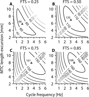
Figure 8: Predicted maximally attainable AMPO as a function of cycle frequency and MTC length excursion, shown for four distinct FTS values. The maximally attainable AMPO (in mW), averaged across three rats, are is depicted as contour lines. The open triangles indicate the location of peak AMPO at each FTS corresponding to the optimal combination of cycle frequency and MTC length excursion for each FTS, with the corresponding peak AMPO labelled at the top-left of the triangle

Figure 9

#%% Load packages & set directories
import os, sys, pickle
import pandas as pd
import numpy as np
from scipy import integrate
import matplotlib.pyplot as plt
from pathlib import Path

# Set directories
cwd = Path.cwd()
baseDir = cwd.parent
dataDir = baseDir / 'data'
funcDir = baseDir / 'analysis' / 'functions'
sys.path.append(str(funcDir))

import cust_fig

plt.close('all')

#%%
customlay = cust_fig.style(plt, fontname='Minion Pro',fontsize=11,grid='false')

fig = plt.figure(figsize=(15.92/2.54+1/600, 11.9/2.54), constrained_layout=True) # 3:2 ratio  
gs = fig.add_gridspec(3,3)
# fig.set_constrained_layout_pads(w_pad=0, h_pad=0, hspace=0, wspace=0)
fig.set_constrained_layout_pads(w_pad=0, h_pad=0, hspace=0, wspace=0.1)
axs = np.array([[fig.add_subplot(gs[i, j]) for j in range(gs.ncols)] for i in range(gs.nrows)])

#%%
nInterpol = 100
colorSet = plt.rcParams['axes.prop_cycle'].by_key()['color']
colorSet[0] = '#000000'
plt.rcParams['axes.prop_cycle'] = plt.cycler('color', colorSet)

symbols = ['o','^', 's']
markersize = 3
for iMus,mus in enumerate(['GMe1', 'GMe2',  'GMe3']):
    dataDirSim = os.path.join(dataDir,mus,'simsCV','')
    parFile = os.path.join(dataDir,mus,mus+'_IM.pkl')
    muspar = pickle.load(open(parFile, 'rb'))[0]
    
    sf = muspar['fmax']*muspar['lce_opt']*1e3
    sf = 1
    
    #%% Imposed CF
    cf_set = np.arange(1.0,6.1,0.5)
    AMPO, cf_imposed, fts_opt, mle_opt = [], [], [], []
    for cf in cf_set:
        try:
            fileName = mus+f'_cf{cf:0.1f}Hz_ftsOpt_mleOpt'
            
            df = pd.read_csv(dataDirSim+fileName+'.csv')
            data = df.to_numpy()
            time,lmtc,_,fsee = data.T[0:4]
            Wmech = -integrate.trapezoid(fsee,lmtc) # [J]
            AMPO.append(Wmech*cf) # [W]
            
            cf_imposed.append(cf)
            fts_opt.append(np.argmin(lmtc)/(len(lmtc)-1)) # [ ]
            mle_opt.append((np.max(lmtc)-np.min(lmtc))) # [m]
        except:
            None
            
    AMPO = np.array(AMPO)/sf
    cf_imposed = np.array(cf_imposed)
    fts_opt = np.array(fts_opt)
    mle_opt = np.array(mle_opt)  
      
    axs[0,0].plot(cf_imposed,AMPO*1e3,color=colorSet[iMus],marker=symbols[iMus],ms=markersize,clip_on=False)
    axs[1,0].plot(cf_imposed,fts_opt,color=colorSet[iMus],marker=symbols[iMus],ms=markersize,clip_on=False)
    axs[2,0].plot(cf_imposed,mle_opt*1e3,color=colorSet[iMus],marker=symbols[iMus],ms=markersize,clip_on=False)
    
    #%% Imposed FTS
    fts_set = [0.25, 0.30, 0.35, 0.40, 0.45, 0.50, 0.55, 0.60, 0.65, 0.70, 0.75, 0.80, 0.85, 0.90, 0.95]
    AMPO, fts_imposed, cf_opt, mle_opt = [], [], [], []
    for fts in fts_set:
        try:
            fileName = mus+f'_cfOpt_fts{fts:{"0.2f"}}_mleOpt'
        
            df = pd.read_csv(dataDirSim+fileName+'.csv')
            data = df.to_numpy()
            time,lmtc,stim,fsee = data.T[0:4]
            Wmech = -integrate.trapezoid(fsee,lmtc) # [J]
            AMPO.append(Wmech/time[-1]) # [W]
            
            fts_imposed.append(fts)
            cf_opt.append(1/time[-1])
            mle_opt.append((np.max(lmtc)-np.min(lmtc))) # [m]
        except:
            None
    
    AMPO = np.array(AMPO)/sf
    fts_imposed = np.array(fts_imposed)
    cf_opt = np.array(cf_opt)
    mle_opt = np.array(mle_opt)
    
    axs[0,1].plot(fts_imposed,AMPO*1e3,color=colorSet[iMus],marker=symbols[iMus],ms=markersize,clip_on=False)
    axs[1,1].plot(fts_imposed,mle_opt*1e3,color=colorSet[iMus],marker=symbols[iMus],ms=markersize,clip_on=False)
    axs[2,1].plot(fts_imposed,cf_opt,color=colorSet[iMus],marker=symbols[iMus],ms=markersize,clip_on=False)
    
    #%% Imposed MLE
    mle_set = np.arange(2,11.1,1)*1e-3
    AMPO, mle_imposed, cf_opt, fts_opt = [], [], [], []
    for mle in mle_set:
        try:
            fileName = mus+f'_cfOpt_ftsOpt_mle{mle*1e3:{"0.1f"}}mm'
            df = pd.read_csv(dataDirSim+fileName+'.csv')
            data = df.to_numpy()
            time,lmtc,stim,fsee = data.T[0:4]
            Wmech = -integrate.trapezoid(fsee,lmtc) # [J]
            AMPO.append(Wmech/time[-1]) # [W]
            
            mle_imposed.append(mle)
            cf_opt.append(1/time[-1])
            fts_opt.append(np.argmin(lmtc)/(len(lmtc)-1)) # [ ]
        except:
            continue
    
    AMPO = np.array(AMPO)/sf
    mle_imposed = np.array(mle_imposed)
    cf_opt = np.array(cf_opt)
    fts_opt = np.array(fts_opt)
        
    axs[0,2].plot(mle_imposed*1e3,AMPO*1e3,color=colorSet[iMus],marker=symbols[iMus],ms=markersize,clip_on=False)
    axs[1,2].plot(mle_imposed*1e3,cf_opt,color=colorSet[iMus],marker=symbols[iMus],ms=markersize,clip_on=False)
    axs[2,2].plot(mle_imposed*1e3,fts_opt,color=colorSet[iMus],marker=symbols[iMus],ms=markersize,clip_on=False)
    
#%%
legend = axs[1,2].legend(['1', '2', '3'],
                       title='Rat',
                       title_fontproperties={'weight': 'bold'},
                       loc='upper right',
                       bbox_to_anchor=(1.05, 1.06),
                       alignment='right',
                       handlelength=0.8,
                       handletextpad=0.5,
                       labelspacing=0.2)

# Effect of CF
for ax in axs[:,0]:
    ax.set_xlim(1,6)
    ax.set_xticks([2,4,6])
    ax.set_xticks([1,3,5], minor=True)

# Effect of FTS
for ax in axs[:,1]:
    ax.set_xlim(0.25,1)
    ax.set_xticks([0.25,0.50,0.75,1.00])
    ax.set_xticks([0.375,0.625,0.875], minor=True)

# Effect of MLE
for ax in axs[:,2]:
    ax.set_xlim(2,11)
    ax.set_xticks([2,6,10])
    ax.set_xticks([4,8], minor=True)

# Effect on AMPO
for ax in axs[0,:]:
    ax.set_ylim(37.5,187.5)
    ax.set_yticks([50,100,150])
    ax.set_yticks([75,125,175], minor=True)

# Effect on FTS
for ax in [axs[1,0], axs[2,2]]:
    ax.set_ylim(0.835,0.885)
    ax.set_yticks([0.84,0.86,0.88])
    ax.set_yticks([0.85,0.87], minor=True)
ax = axs[1,0]
ax.set_ylim(0.835,0.885)
ax.set_yticks([0.84,0.86,0.88])
ax.set_yticks([0.85,0.87], minor=True)
ax = axs[2,2]
ax.set_ylim(0.835,0.855)
ax.set_yticks([0.84,0.85])
ax.set_yticks([0.845], minor=True)

# Effect on MLE
for ax in [axs[1,1], axs[2,0]]:
    ax.set_ylim(4.5,11.5)
    ax.set_yticks([6,8,10])
    ax.set_yticks([5,7,9], minor=True)
ax = axs[1,1]
ax.set_ylim(4.5,9)
ax.set_yticks([6,8])
ax.set_yticks([5,7,9], minor=True)
ax = axs[2,0]
ax.set_ylim(3.5,13.5)
ax.set_yticks([4,8,12])
ax.set_yticks([6,10], minor=True)

# Effect on CF
for ax in [axs[1,2], axs[2,1]]:
    ax.set_ylim(1,9)
    ax.set_yticks([2,4,6,8])
    ax.set_yticks([1,3,5,7,9], minor=True)
ax = axs[1,2]
ax.set_ylim(2.5,9.5)
ax.set_yticks([4,6,8])
ax.set_yticks([3,5,7,9], minor=True)
ax = axs[2,1]
ax.set_ylim(1.75,4.25)
ax.set_yticks([2,3,4])
ax.set_yticks([2.5,3.5], minor=True)

#%% Labels etc.
axs[2,0].set_xlabel('CF [Hz]')
axs[2,1].set_xlabel('FTS [ ]')
axs[2,2].set_xlabel('$\Delta L_{MTC}$ [mm]')
axs[0,0].set_ylabel('AMPO [mW]')
axs[0,1].set_ylabel('AMPO [mW]')
axs[0,2].set_ylabel('AMPO [mW]')
axs[1,0].set_ylabel('FTS [ ]')
axs[2,0].set_ylabel('$\Delta L_{MTC}$ [mm]')
axs[1,1].set_ylabel('$\Delta L_{MTC}$ [mm]')
axs[2,1].set_ylabel('CF [Hz]')
axs[1,2].set_ylabel('CF [Hz]')
axs[2,2].set_ylabel('FTS [ ]')

for ax in axs.flatten():
    ax.spines['left'].set_position(('outward', 12)) 
    ax.yaxis.labelpad = 0

fig.align_labels()

#%%
labels = ['A1','B1','C1', 'A2','B2','C2', 'A3','B3','C3']
cust_fig.add_labels(fig, axs.flatten(), labels, -15/72)
    
# %% Show and save
plt.show()
# # fig.savefig("r_interrelationships.png", bbox_inches="tight", pad_inches=0, dpi=600)
fig.savefig("r_interrelationships.pdf", bbox_inches="tight", pad_inches=0)
# # fig.savefig("r_interrelationships.svg", bbox_inches="tight", pad_inches=0)

# %% Checks
if len(sys.argv) > 1:
    check_size = sys.argv[1]
else:
    check_size = True  

if check_size == True or check_size == 'True':
    cust_fig.report_axes_size(fig,axs)
    # cust_fig.report_fig_size("r_interrelationships.png") 
    cust_fig.report_fig_size("r_interrelationships.pdf") 
    # cust_fig.report_fig_size("r_interrelationships.svg") 

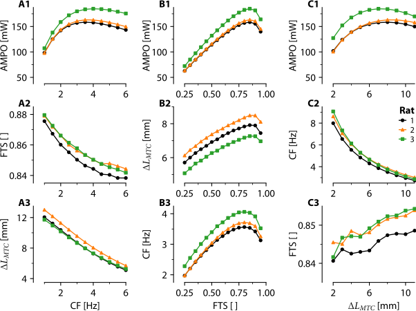
Figure 9: Predicted interrelationships between cycle frequency (CF), FTS, MTC length excursion (MLE) and the maximally attainable AMPO. These plots collectively illustrate how cycle frequency, FTS, and MTC length excursion interact to maximise AMPO under different conditions. This figure presents a 3x3 grid of plots created by imposing one SSC parameter at a time while optimising the two other SSC parameters to maximise AMPO. In the first column, cycle frequency was imposed, and AMPO (A1) was maximised by identifying the optimal FTS (A2) and MTC length excursion (A3) at each cycle frequency. In the second column, FTS was imposed, and AMPO (A1) was maximised by identifying the optimal MTC length excursion (B2) and cycle frequency (B3) at FTS. In the third column, MTC length excursion was imposed, and AMPO (C1) was maximised by identifying the optimal cycle frequency (C2) and FTS (C3) at each MTC length excursion. For all columns, muscle stimulation onset time and duration were optimised to maximise AMPO.

Figure 10

#%% Load packages & set directories
import os, sys, pickle
import numpy as np
import pandas as pd
import matplotlib.pyplot as plt
from pathlib import Path

# Set directories
cwd = Path.cwd()
baseDir = cwd.parent
dataDir = baseDir / 'data'
funcDir = baseDir / 'analysis' / 'functions'
sys.path.append(str(funcDir))

import cust_fig, hillmodel

plt.close('all')

#%%
cust_fig.style(plt, fontname='Minion Pro',fontsize=11,grid=False)
# fig = plt.figure(figsize=(15.92/2.54+0.085, 13.36/2.54), constrained_layout=True) # 3:2 ratio
fig = plt.figure(figsize=(15.92/2.54+0.085, 14.90/2.54), constrained_layout=True) # 3:2 ratio
# fig = plt.figure(figsize=(15.92/2.54+0.085, 15.92/2.54/3+0.085), constrained_layout=True) # 3:1 ratio
gs = fig.add_gridspec(6, 2, height_ratios=[1e-3,1.02,8.4,8.4,1e-3,8.4], wspace=0)
axs = np.array([[fig.add_subplot(gs[i, j]) for j in range(gs.ncols)] for i in range(gs.nrows)])
axs = axs.flatten().tolist()

# These are 'fake axis' to create title above the two 'blocks'
axs[9].remove(); del(axs[9])
axs[8].remove(); del(axs[8])
axs[1].remove(); del(axs[1])
axs[0].remove(); del(axs[0])

#%% Subplot 1,1
mus = 'GMe1'
parFile = os.path.join(dataDir,mus,mus+'_IM.pkl')
muspar = pickle.load(open(parFile, 'rb'))[0]
musparLong  = muspar.copy()
musparShort = muspar.copy()
muspar_lsee0_new = 3e-3
musparShort['ksee'] = musparShort['ksee']*(musparShort['lsee0']/muspar_lsee0_new)**2
musparShort['lsee0'] = muspar_lsee0_new
dataDirSim = os.path.join(dataDir,mus,'simsOC','')
fmax, lce_opt = muspar['fmax'], muspar['lce_opt']

cfSet = [2.5, 3.5, 4.5]
cfSet = [2.0, 3.5, 5]

colorSet = plt.rcParams['axes.prop_cycle'].by_key()['color']
colorSet[0] = colorSet[1]
colorSet[1] = '#000000'
# colorSet[1] = '#1f77b4'
for idx,cf in enumerate(cfSet):
    fileName = mus+f'_cf{cf:{"0.1f"}}Hz_ftsOpt_mleOpt'  
    df = pd.read_csv(dataDirSim+fileName+'.csv', sep=',')
    data = df.to_numpy()
    time,lmtc,stim,fsee,gamma,lcerel = data.T[0:6]
    
    lce = lcerel*lce_opt
    vce = np.gradient(lce,time)
       
    time = time/time[-1]
    time = np.concatenate((time-time[-1],time,time+time[-1]))
    lce = np.concatenate((lce,lce,lce))
    fsee = np.concatenate((fsee,fsee,fsee))
    vce = np.concatenate((vce,vce,vce))
    stim = np.concatenate((stim,stim,stim))
    lpee = lce
    fpee = hillmodel.lee2force(0,lpee,muspar)[1]
    fce = fsee-fpee
    IMPO = -fce*vce
    
    stim[stim>=0.5] = 1.0; 
    stim[stim<0.5] = 0
    tStimOn = time[np.where(np.diff(stim)>0.1)[0]]
    tStimOff = time[np.where(np.diff(stim)<-0.1)[0]]
    cust_fig.plot_stim(axs[0],tStimOn[0],tStimOff[1],y=-idx, lw=1/3, color=colorSet[idx])
    cust_fig.plot_stim(axs[0],tStimOn[1],tStimOff[2],y=-idx, lw=1/3 ,color=colorSet[idx])
    
    # Lmtc(t): Long SEE
    lseeLong = hillmodel.force2lee(fsee,fpee,musparLong)[0]
    lmtcLong = lce + lseeLong

    # Lmtc(t): Short SEE
    lseeShort = hillmodel.force2lee(fsee,fpee,musparShort)[0]
    lmtcShort = lce + lseeShort
    
    # plotStim(axs[1],tStimOn[0],tStimOff[1],y=-idx, lw=1/3, color=colorSet[idx])
    # plotStim(axs[1],tStimOn[1],tStimOff[2],y=-idx, lw=1/3 ,color=colorSet[idx])
    
    axs[1].plot(time,stim, color=colorSet[idx]) # plotted but not visible!
    
    if tStimOff[-1] > 1.75: 
        print('Warning, tStimoff exceed plotted values!!')
    
    axs[2].plot(time,lce*1e3, color=colorSet[idx])
    axs[3].plot(time,fce, color=colorSet[idx])
    axs[4].plot(time,vce*1e3, color=colorSet[idx])
    axs[5].plot(time,IMPO*1e3, color=colorSet[idx])
    
    axs[6].plot(time,lmtcLong*1e3, color=colorSet[idx])
    axs[7].plot(time,lmtcShort*1e3, color=colorSet[idx])
  
legend = axs[1].legend(["2.0 Hz", "3.5 Hz", "5.0 Hz"],
                       loc='center',
                       ncol=3,
                       bbox_to_anchor=(0.5, 0.5),  # slight offset above the axes
                       handlelength=0.8,
                       handletextpad=0.5,
                       labelspacing=0.2)


for ax in [axs[0], axs[1], axs[2], axs[3], axs[4], axs[5], axs[6], axs[7]]:
    ax.set_xlim(-0.25,1.75)

# stim(t)
# axs[0].autoscale(enable=True, axis='y', tight=True)
axs[0].set_ylim(-7/3,1/3)
axs[0].spines['top'].set_visible(False)
axs[0].spines['right'].set_visible(False)
axs[0].spines['bottom'].set_visible(False)
axs[0].spines['left'].set_visible(False)
axs[0].set_xticks([]);
axs[0].set_yticks([]); 
axs[1].autoscale(enable=True, axis='y', tight=True)
axs[1].set_ylim(500,900) # range way outside what is plotted, only for legend purpose!
axs[1].spines['top'].set_visible(False)
axs[1].spines['right'].set_visible(False)
axs[1].spines['bottom'].set_visible(False)
axs[1].spines['left'].set_visible(False)
axs[1].set_xticks([]);
axs[1].set_yticks([]); 

# lce(t)    
axs[2].set_ylim(7,20)
axs[2].set_yticks([10,14,18])
axs[2].set_yticks([12,16],minor=True)
axs[2].set_ylabel('CE length [mm]')
ax2T = axs[2].twinx()
ax2T.spines['right'].set_visible(True)
ax2T.plot(time,lce/lce_opt, linewidth=1, linestyle ='--', color='k', alpha=0)
ax2T.set_ylim((axs[2].get_ylim()[0]/1e3/lce_opt, axs[2].get_ylim()[1]/1e3/lce_opt)) 
ax2T.set_yticks([0.6,1.0,1.4])
ax2T.set_yticks([0.8,1.2],minor=True)
ax2T.set_ylabel('$L_{CE}^{rel}$ [ ]')
 
# fsee(t)
ax = axs[3]
ax.set_ylim(0,11)
ax.set_yticks([0,4,8])
ax.set_yticks([2,6],minor=True)
ax.set_ylabel('CE force [N]')
axFsee = ax.twinx()
axFsee.spines['right'].set_visible(True)
axFsee.plot(time,fce/fmax, linewidth=1, linestyle ='--', color='k', alpha=0)
axFsee.set_ylim((ax.get_ylim()[0]/fmax, ax.get_ylim()[1]/fmax)) 
axFsee.set_yticks([0,0.2,0.4,0.6])
axFsee.set_yticks([0.1,0.3,0.5,0.7],minor=True)
axFsee.set_ylabel('$F_{CE}^{rel}$ [ ]')

# vce(t)
ax = axs[4]
ax.set_ylim(-75,270)
ax.set_yticks([0,100,200])
ax.set_yticks([-50,50,150,250],minor=True)
ax.set_ylabel('CE velocity [mm/s]')
axVce = ax.twinx()
axVce.spines['right'].set_visible(True)
axVce.plot(time,vce/lce_opt, linewidth=1, linestyle ='--', color='k', alpha=0)
axVce.set_ylim((ax.get_ylim()[0]/1e3/lce_opt, ax.get_ylim()[1]/1e3/lce_opt)) 
axVce.set_yticks([0,8,16])
axVce.set_yticks([-4,4,12],minor=True)
axVce.set_ylabel('$V_{CE}^{rel}$ [1/s]')

# IMPO(t)
ax = axs[5]
ax.set_ylim(-350,350)
ax.set_yticks([-200,0,200])
ax.set_yticks([-300,-100,0,100,300],minor=True)
ax.set_ylabel('IMPO [mW]')
axImpo = ax.twinx()
axImpo.spines['right'].set_visible(True)
axImpo.plot(time,IMPO/(lce_opt*fmax), linewidth=1, linestyle ='--', color='k', alpha=0)
axImpo.set_ylim((ax.get_ylim()[0]/1e3/(lce_opt*fmax), ax.get_ylim()[1]/1e3/(lce_opt*fmax))) 
axImpo.set_yticks([-1,0,1])
axImpo.set_yticks([-1.5,-0.5,0.5,1.5],minor=True)
# axImpo.set_ylabel(r'$\frac{\mathrm{IMPO}}{L_{CE}^{opt} \cdot F_{CE}^{max}}$ [1/s]')
axImpo.set_ylabel(    r'$\frac{\mathsf{IMPO}}{L_{CE}^{opt}\cdot F_{CE}^{max}}$ [1/s]', usetex=True)

# Lmtc Long (t)
ax = axs[6]
ax.set_title('Typical SEE slack length (28 mm)', loc="left")
ax.set_ylim(38,51)
ax.set_yticks([40,44,48])
ax.set_yticks([42,46,50],minor=True)
ax.set_ylabel('MTC length [mm]')

# Lmtc Long (t)
ax = axs[7]
ax.set_title('Short SEE slack length (3 mm)', loc="left")
ax.set_ylim(10,23)
ax.set_yticks([12,16,20])
ax.set_yticks([10,14,18,22],minor=True)
ax.set_ylabel('MTC length [mm]')

axs[2].plot([-2,2],[lce_opt*1e3,lce_opt*1e3],'k--',alpha=0.25,lw=0.5,zorder=-100)
axs[4].plot([-2,2],[0,0],'k--',alpha=0.25,lw=0.5,zorder=-100)
axs[5].plot([-2,2],[0,0],'k--',alpha=0.25,lw=0.5,zorder=-100)

# axs[4].set_xlabel('Normalised time [s]')
# axs[5].set_xlabel('Normalised time [s]')
axs[6].set_xlabel('Normalised time [s]')
axs[7].set_xlabel('Normalised time [s]')

axsTitle = fig.add_subplot(gs[0, :])
axsTitle.set_title('CE Dynamics', fontweight='bold', fontsize='large')
axsTitle.set_frame_on(False)
axsTitle.axis('off')

axsTitle = fig.add_subplot(gs[4, :])
axsTitle.set_title('MTC Dynamics', fontweight='bold', fontsize='large')
axsTitle.set_frame_on(False)
axsTitle.axis('off')

fig.align_labels()
cust_fig.add_labels(fig, axs, ['', '', 'A', 'B', 'C', 'D', 'E', 'F'])

# %% Show and save
plt.show()
# fig.savefig("r_oc.png", bbox_inches="tight", pad_inches=0, dpi=600)
fig.savefig("r_oc.pdf", bbox_inches="tight", pad_inches=0)
# fig.savefig("r_oc.svg", bbox_inches="tight", pad_inches=0)

# %% Checks
if len(sys.argv) > 1:
    check_size = sys.argv[1]
else:
    check_size = True  

if check_size == True or check_size == 'True':
    cust_fig.report_axes_size(fig,axs)
    # cust_fig.report_fig_size("r_oc.png") 
    cust_fig.report_fig_size("r_oc.pdf") 
    # cust_fig.report_fig_size("r_oc.svg")

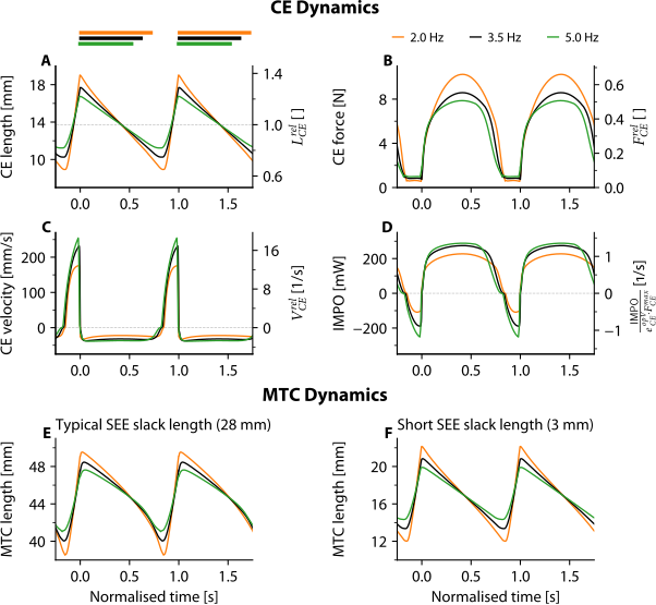
Figure 10: Predicted CE behaviour for maximally attainable AMPO, shown at three distinct cycle frequencies for rat 1. CE length (A), CE force (B), CE velocity (C) and instantaneous mechanical power output (IMPO) (D) as a function of normalised time (i.e. time divided by the cycle duration). CE stimulation was maximal during the period indicated by the coloured bars and fully off elsewhere. The right labels depict the normalised values, where CE length and CE velocity are normalised to optimum CE length, CE force is normalised to maximal isometric CE force and IMPO is normalised to the product of optimum CE length and maximal isometric CE force. Based on CE length and force over time, and the SEE properties, the MTC length over time can be calculated. The resulting MTC length over time substantially differs between a typical SEE slack length of 28 mm (E) and a short SEE slack length of 3 mm (F).

Supplementary material

Figure S1

#%%
import os, sys
import numpy as np
import matplotlib.pyplot as plt
from pathlib import Path

# Set directories
cwd = Path.cwd()
baseDir = cwd.parent
dataDir = baseDir / 'data'
funcDir = baseDir / 'analysis' / 'functions'
sys.path.append(str(funcDir))

import cust_fig, helpers, interpolation

plt.close('all')

#%% Make figure
customlay = cust_fig.style(plt, fontname='Minion Pro',fontsize=11,grid=False)
customlay['xtick.direction'] = 'out' # cause of contour plot
customlay['ytick.direction'] = 'out'
# plt.rcParams.update(plt.rcParamsDefault)
plt.rcParams.update(customlay)

fig = plt.figure(figsize=(15.92/2.54+51/600, (15.92/2-1.6)/2.54), constrained_layout=True) # 3:2 ratio
gs = fig.add_gridspec(1,2)
# axs = [fig.add_subplot(gs[i]) for i in range(0,gs.ncols*gs.nrows)]
axs = [fig.add_subplot(gs[0, 0])]
axs.append(fig.add_subplot(gs[0, 1]))

#%% Loop
ftsSet = np.arange(0.05, 0.96, 0.05)
for iAmp, amp in enumerate([2e-3 , 4e-3]):
    if amp == 2e-3:
        cfSet = np.arange(0.4, 6.1, 0.2)
    elif amp == 4e-3:
        cfSet = np.arange(0.4, 4.1, 0.2)
    else:
        breakpoint()
    AMPOsets, AMPOfines, sf = [], [], []
    for iMus,mus in enumerate(['GMz1', 'GMz2', 'GMz3']):
        # Load muspar
        # parFile = os.path.join(dataDir,mus,mus+'_IM.pkl')
        # muspar = pickle.load(open(parFile, 'rb'))[0]
        # sf.append(muspar['lce_opt']*muspar['fmax'])
        sf.append(1)
    
        filepaths = [[os.path.join(dataDir,'prelim', mus, f'{mus}_amp{amp*1e3:0.1f}mm_cf{cf:0.1f}Hz_fts{fts:0.2f}.csv') for fts in ftsSet] for cf in cfSet] 
        AMPOset = helpers.get_ampo(filepaths)
        AMPOfine,(cfFine,ftsFine) = interpolation.do_3d(AMPOset,(cfSet,ftsSet),N=19,method='cubic')
           
        # Append to list for all muscles
        AMPOset = AMPOset/sf[iMus]
        AMPOsets.append(AMPOset)
        AMPOfine = AMPOfine/sf[iMus]
        AMPOfines.append(AMPOfine)
    
    #%% Calculate average   
    AMPOsets        = np.dstack(AMPOsets)
    AMPOfines       = np.dstack(AMPOfines)
    meanAMPOsets    = np.mean(AMPOsets,2)
    meanAMPOsets    = meanAMPOsets*np.mean(sf)
    meanAMPOfines   = np.mean(AMPOfines,2)
    meanAMPOfines   = meanAMPOfines*np.mean(sf)
    
    #%% Make figure 
    AMPOmax = np.nanmax(AMPOfine)
    contour_levels  = np.arange(10,AMPOmax*1e3,10)
    
    cmap = plt.get_cmap('gray_r')
    cmap = cust_fig.truncate_colormap(cmap, 0.25, 1)
    
    iAx = iAmp
    CS = axs[iAx].contour(cfFine,ftsFine,AMPOfine*1e3,contour_levels,cmap=cmap)
    
    x1, x2 = 0.5, [6,4][iAmp]
    y1, y2 = 0.05, 0.95
    
    a = (y2 - y1) / (x2 - x1)
    b = y1 - a * x1
    
    def line_func(x):
        return a * x + b

    # Function to compute intersection between segment and line
    def segment_line_intersection(p1, p2, a, b):
        x1, y1 = p1
        x2, y2 = p2
        # Represent line segment as p + t*r, intersect with line y = ax + b
        denom = (y2 - y1) - a * (x2 - x1)
        if denom == 0:
            return None  # Parallel
        t = ((a * x1 + b) - y1) / denom
        if 0 <= t <= 1:
            x_int = x1 + t * (x2 - x1)
            y_int = y1 + t * (y2 - y1)
            if np.isclose(y_int, a * x_int + b):
                return x_int, y_int
        return None

    # Find intersection points to use for manual labels
    manual_locations = []

    for i, segs in enumerate(CS.allsegs):
        for seg in segs:
            for j in range(len(seg) - 1):
                p1, p2 = seg[j], seg[j + 1]
                pt = segment_line_intersection(p1, p2, a, b)
                if pt is not None:
                    manual_locations.append(pt)
    # if fts == 0.50:
    #     del(manual_locations[11])
    #     del(manual_locations[10])
    
    
    if manual_locations:
        axs[iAx].clabel(CS, fmt = '%2.0f',fontsize=9, manual=manual_locations)
    
#%%    
fig.supxlabel('Cycle frequency [Hz]', fontsize=11)
fig.supylabel('FTS [ ]', fontsize=11)

axs[0].set_title('MTC length excursion = 4 mm')
axs[1].set_title('MTC length excursion = 8 mm')

for ax in axs:
    ax.set_ylim(0.05,0.95)
    ax.set_xticks([1.0,2.0,3.0,4.0,5.0,6.0])
    ax.set_xticks([1.5,2.5,3.5,4.5,5.5], minor=True)   
    # ax.set_yticks([2.0,4.0,6.0,8.0,10])
    # ax.set_yticks([3,5,7,9,11], minor=True)

axs[0].set_xlim(0.5,6)
axs[1].set_xlim(0.5,4) 

cust_fig.add_labels(fig, axs, ['A','B'])

# %% Show and save
plt.show()
# fig.savefig("s_prelim.png", bbox_inches="tight", pad_inches=0, dpi=600)
fig.savefig("s_prelim.pdf", bbox_inches="tight", pad_inches=0)
# fig.savefig("s_prelim.svg", bbox_inches="tight", pad_inches=0)

# %% Checks
if len(sys.argv) > 1:
    check_size = sys.argv[1]
else:
    check_size = True  

if check_size == True or check_size == 'True':
    cust_fig.report_axes_size(fig,axs)
    # cust_fig.report_fig_size("s_prelim.png") 
    cust_fig.report_fig_size("s_prelim.pdf") 
    # cust_fig.report_fig_size("s_prelim.svg")

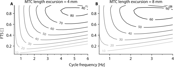
Figure S1: Preliminary predictions of maximal AMPO as a function of cycle frequency and FTS. The contour lines depict the maximally attainable AMPO (in mW) averaged over three parameter sets. These preliminary predictions were derived with a Hill-type MTC model with parameters obtained from literature (Zandwijk et al. 1996) and were used to inform the selection of experimental SSC conditions.

Figure S2

#%%
import os, sys, pickle
import numpy as np
import pandas as pd
import matplotlib.pyplot as plt
from pathlib import Path

# Set directories
cwd = Path.cwd()
baseDir = cwd.parent
dataDir = baseDir / 'data'
funcDir = baseDir / 'analysis' / 'functions'
sys.path.append(str(funcDir))

import cust_fig, stimulation

plt.close('all')

#%% Select rat
mus = 'GMe1'
parFile = os.path.join(dataDir,mus,mus+'_IM.pkl')
muspar = pickle.load(open(parFile, 'rb'))[0]
dataDirSim = os.path.join(dataDir,mus,'simsOC','')

#%%
cust_fig.style(plt, fontname='Minion Pro',fontsize=11,grid=False)
fig = plt.figure(figsize=(15.92/2.54+50/600, 5.4/2.54), constrained_layout=True) # 3:2 ratio
gs = fig.add_gridspec(2, 2, height_ratios=[1/10.97,1], wspace=0.3/3)
axs = [fig.add_subplot(gs[i]) for i in range(0,gs.ncols*gs.nrows)]

colorSet = plt.rcParams['axes.prop_cycle'].by_key()['color']
colorSet[0] = '#000000'

#%% Impsed FTS (&CF)
cf = 3.5
for iFts,fts in enumerate([0.5, 0.95]):
    fileName = mus+f'_cf{cf:0.1f}Hz_fts{fts:0.2f}_mleOpt'
    
    # Experimental data
    df = pd.read_csv(dataDirSim+fileName+'.csv')
    data = df.to_numpy()
    time,lmtc,stim,fsee,gamma,lcerel = data.T[0:6]
    time = np.concatenate((time-time[-1],time,time+time[-1]))
    lcerel = np.concatenate((lcerel,lcerel,lcerel))
    lce = lcerel*muspar['lce_opt']*1e3
    stim = np.concatenate((stim,stim,stim))
    
    # Plot STIM(t)
    tStimOn, tStimOff = stimulation.get_stim_timing(time,stim)
    cust_fig.plot_stim(axs[0],tStimOn[0],tStimOff[0],y=iFts, lw=1/3, color=colorSet[iFts])
    cust_fig.plot_stim(axs[0],tStimOn[1],tStimOff[1],y=iFts, lw=1/3, color=colorSet[iFts])
    cust_fig.plot_stim(axs[0],tStimOn[2],tStimOff[2],y=iFts, lw=1/3, color=colorSet[iFts])

    # Plot Lce(t)
    axs[2].plot(time,lce, color=colorSet[iFts], label=f'{fts:.2f}')

axs[2].set_ylim(8, 20)
ax2T = axs[2].twinx()
ax2T.spines['right'].set_visible(True)
scale_factor = muspar['lce_opt']*1000
y1_min, y1_max = axs[2].get_ylim()
ax2T.set_ylim(y1_min / scale_factor, y1_max / scale_factor)
# ax2T.plot(time,lcerel)

#%% Impsed AMP (&CF)
cf = 3.5
for iFts,mle in enumerate([2, 10]):
    fileName = mus+f'_cf{cf:0.1f}Hz_ftsOpt_mle{mle:04.1f}mm'
    
    # Experimental data
    df = pd.read_csv(dataDirSim+fileName+'.csv')
    data = df.to_numpy()
    time,lmtc,stim,fsee,gamma,lcerel = data.T[0:6]
    time = np.concatenate((time-time[-1],time,time+time[-1]))
    lcerel = np.concatenate((lcerel,lcerel,lcerel))
    lce = lcerel*muspar['lce_opt']*1e3
    stim = np.concatenate((stim,stim,stim))
    
    # Plot STIM(t)
    tStimOn, tStimOff = stimulation.get_stim_timing(time,stim)
    cust_fig.plot_stim(axs[1],tStimOn[0],tStimOff[0],y=iFts, lw=1/3, color=colorSet[iFts])
    cust_fig.plot_stim(axs[1],tStimOn[1],tStimOff[1],y=iFts, lw=1/3, color=colorSet[iFts])
    cust_fig.plot_stim(axs[1],tStimOn[2],tStimOff[2],y=iFts, lw=1/3, color=colorSet[iFts])
    
    # Plot Lce(t)
    axs[3].plot(time,lce, color=colorSet[iFts], label=f'{mle:.2f}')

axs[3].set_ylim(8,20)
ax3T = axs[3].twinx()
ax3T.spines['right'].set_visible(True)
scale_factor = muspar['lce_opt']*1000
y1_min, y1_max = axs[3].get_ylim()
ax3T.set_ylim(y1_min / scale_factor, y1_max / scale_factor)
# ax3T.plot(time,lcerel)

#%% Legends
axs[2].legend(['0.50', '0.95'],
    title='FTS',
    title_fontproperties={'weight': 'bold'},
    loc='upper right',
    bbox_to_anchor=(0.98, 1.2),  # shift left (into space between axes) and center vertically
    frameon=False,
    handlelength=1,
    handletextpad=0.5,
    labelspacing=0.2,
    alignment='right'
)


axs[3].legend(['2 mm', '10 mm'],
    title='MTC length excursion',
    title_fontproperties={'weight': 'bold'},
    loc='upper right',
    bbox_to_anchor=(1.03, 1.2),  # shift left (into space between axes) and center vertically
    frameon=False,
    handlelength=1,
    handletextpad=0.5,
    labelspacing=0.2,
    alignment='right',
)

#%% Labels etc.
# STIM(t)
for ax in axs[0:2]:
    ax.set_xlim(-0.25/3.5,1.75/3.5)
    ax.spines['top'].set_visible(False)
    ax.spines['right'].set_visible(False)
    ax.spines['bottom'].set_visible(False)
    ax.spines['left'].set_visible(False)
    ax.set_xticks([])
    ax.set_yticks([])
    ax.autoscale(enable=True, axis='y', tight=True)
  
# Lmtc(t)
for ax in axs[2:]:
    ax.set_xlim(-0.25/3.5,1.75/3.5)
    ax.set_xticks([0,0.2,0.4])
    ax.set_xticks([0.1,0.3,0.5],minor=True)
    # ax.set_ylim(8.5,19.5)
    ax.set_yticks([10,14,18])
    ax.set_yticks([12,16],minor=True)
    ax.set_ylabel('$L_{CE}$ [mm]')
    
for ax in [ax2T, ax3T]:
    ax.set_yticks([0.6,1.0,1.4])
    ax.set_yticks([0.8,1.2],minor=True)
    ax.set_ylabel('$L_{CE}^{rel}$ [ ]')

axs[2].set_xlabel('Time [s]')
axs[3].set_xlabel('Time [s]')

fig.align_labels()
cust_fig.add_labels(fig, axs, ['','','A','B'])

# %% Show and save
plt.show()
# fig.savefig("s_oc.png", bbox_inches="tight", pad_inches=0, dpi=600)
fig.savefig("s_oc.pdf", bbox_inches="tight", pad_inches=0)
# fig.savefig("s_oc.svg", bbox_inches="tight", pad_inches=0)

# %% Checks
if len(sys.argv) > 1:
    check_size = sys.argv[1]
else:
    check_size = True  

if check_size == True or check_size == 'True':
    cust_fig.report_axes_size(fig,axs)
    # cust_fig.report_fig_size("s_oc.png") 
    cust_fig.report_fig_size("s_oc.pdf") 
    # cust_fig.report_fig_size("s_oc.svg")

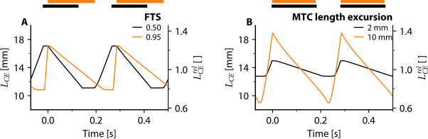
Figure S2: Predicted CE length over time for maximally attainable AMPO, shown for two imposed FTS values (A) and two imposed MTC length excursions (B), at a cycle frequency of 3.5 Hz for rat 1**. In panel A, only cycle frequency and FTS were imposed, while in panel B only cycle frequency and MTC length excursions were imposed. Apart from these two constraints, CE and MTC length over time were completely unconstrained and thus the shape of CE length over time could be different between every combination of imposed cycle frequency and FTS (A) or imposed cycle frequency and MTC length excursion (B). CE stimulation was maximal during the period indicated by the coloured bars, and ‘off’ elsewhere.

Figure S3

#%%
import os,sys
import pandas as pd
import numpy as np
from scipy import integrate
import matplotlib.pyplot as plt
from pathlib import Path

# Set directories
cwd = Path.cwd()
baseDir = cwd.parent
dataDir = baseDir / 'data'
funcDir = baseDir / 'analysis' / 'functions'
sys.path.append(str(funcDir))

import cust_fig

plt.close('all')

#%%
cust_fig.style(plt, fontname='Minion Pro',fontsize=11,grid=False)
fig = plt.figure(figsize=(15.92/2.54, 4.77/2.54), constrained_layout=True) # width & height  
gs = fig.add_gridspec(1,3)
axs = [fig.add_subplot(gs[i]) for i in range(0,gs.ncols*gs.nrows)]

colorSet = plt.rcParams['axes.prop_cycle'].by_key()['color']
colorSet[0] = '#000000'

sf = 1
    
#%% Imposed CF
cfSet = np.arange(1.0,6.1,0.5)
for i,traj in enumerate(['simsCV', 'simsOC']):
    AMPOall = []
    for mus in ['GMe1', 'GMe2', 'GMe3']:
        dataFolder = os.path.join(dataDir,mus,traj,'')
        AMPOmus = []
        for cf in cfSet:
            try:
                filepath = os.path.join(dataFolder, f'{mus}_cf{cf:0.1f}Hz_ftsOpt_mleOpt.csv')
                df = pd.read_csv(filepath)
                data = df.to_numpy()
                time,lmtc,_,fsee = data.T[0:4]
                Wmech = -integrate.trapezoid(fsee,lmtc)*1e3 # [mJ]
                AMPOmus.append(Wmech/time[-1]) # [mW]
            except:
                AMPOmus.append(np.nan)
            
        AMPOmus = np.array(AMPOmus)/sf      
        AMPOall.append(AMPOmus)
    axs[0].plot(cfSet,np.mean(AMPOall,0),'.-',color=colorSet[i],clip_on=False)
    
#%% Imposed FTS
ftsSet = [0.25, 0.30, 0.35, 0.40, 0.45, 0.50, 0.55, 0.60, 0.65, 0.70, 0.75, 0.80, 0.85, 0.88, 0.90, 0.92, 0.95]
ftsSet = [0.25, 0.30, 0.35, 0.40, 0.45, 0.50, 0.55, 0.60, 0.65, 0.70, 0.75, 0.80, 0.85, 0.90, 0.95]
for i,traj in enumerate(['simsCV', 'simsOC']):
    AMPOall = []
    for mus in ['GMe1', 'GMe2', 'GMe3']:
        dataFolder = os.path.join(dataDir,mus,traj,'')
        AMPOmus = []
        for fts in ftsSet:
            try:
                filepath = os.path.join(dataFolder, f'{mus}_cfOpt_fts{fts:0.2f}_mleOpt.csv')
                df = pd.read_csv(filepath)
                data = df.to_numpy()
                time,lmtc,_,fsee = data.T[0:4]
                Wmech = -integrate.trapezoid(fsee,lmtc)*1e3 # [mJ]
                AMPOmus.append(Wmech/time[-1]) # [mW]
            except:
                AMPOmus.append(np.nan)
            
        AMPOmus = np.array(AMPOmus)/sf      
        AMPOall.append(AMPOmus)
    axs[1].plot(ftsSet,np.mean(AMPOall,0),'.-',color=colorSet[i],clip_on=False)
    
#%% Imposed MLE
mleSet = [2, 3, 4, 5, 6, 7, 8, 9, 10, 11]
for i,traj in enumerate(['simsCV', 'simsOC']):
    AMPOall = []
    for mus in ['GMe1', 'GMe2', 'GMe3']:
        dataFolder = os.path.join(dataDir,mus,traj,'')
        AMPOmus = []
        for mle in mleSet:
            try:
                filepath = os.path.join(dataFolder, f'{mus}_cfOpt_ftsOpt_mle{mle:04.1f}mm.csv')
                df = pd.read_csv(filepath)
                data = df.to_numpy()
                time,lmtc,_,fsee = data.T[0:4]
                Wmech = -integrate.trapezoid(fsee,lmtc)*1e3 # [mJ]
                AMPOmus.append(Wmech/time[-1]) # [mW]
            except:
                AMPOmus.append(np.nan)
            
        AMPOmus = np.array(AMPOmus)/sf      
        AMPOall.append(AMPOmus)
    axs[2].plot(mleSet,np.mean(AMPOall,0),'.-',color=colorSet[i],clip_on=False)
    
#%%
leg = axs[2].legend(['Constant', 'Optimal'],
    title='MTC velocities',
    title_fontproperties={'weight': 'bold'},
    loc='lower right',
    bbox_to_anchor=(1.08, 0),  # shift left (into space between axes) and center vertically
    frameon=False,
    handlelength=1,
    handletextpad=0.5,
    labelspacing=0.2,
    alignment='right'
)
    
#%% Labels etc.
axs[0].set_xlabel('Cycle frequency [Hz]')
axs[1].set_xlabel('FTS [ ]')
axs[2].set_xlabel('MTC length excursion [mm]',x=0.395)
axs[0].set_ylabel('AMPO [mW]')
axs[1].set_ylabel('AMPO [mW]')
axs[2].set_ylabel('AMPO [mW]')

axs[0].set_xlim(1,6)
axs[0].set_xticks([2,4,6])
axs[0].set_xticks([1,3,5],minor=True)

axs[1].set_xlim(0.25,1)
axs[1].set_xticks([0.25,0.50,0.75,1.00])
axs[1].set_xticks([0.375,0.625,0.875], minor=True)

ax = axs[2]
ax.set_xlim(2,11)
ax.set_xticks([2,6,10])
ax.set_xticks([4,8], minor=True)

for ax in axs:
    ax.set_ylim(50,175)
    ax.set_yticks([50,100,150])
    ax.set_yticks([75,125,175],minor=True)

for ax in axs:
    ax.spines['left'].set_position(('outward', 12)) 

fig.align_labels()
cust_fig.add_labels(fig, axs, ['A','B','C'], -15/72)

# %% Show and save
plt.show()
# fig.savefig("s_ampo.png", bbox_inches="tight", pad_inches=0, dpi=600)
fig.savefig("s_ampo.pdf", bbox_inches="tight", pad_inches=0)
# fig.savefig("s_ampo.svg", bbox_inches="tight", pad_inches=0)

# %% Checks
if len(sys.argv) > 1:
    check_size = sys.argv[1]
else:
    check_size = True  

if check_size == True or check_size == 'True':
    cust_fig.report_axes_size(fig,axs)
    # cust_fig.report_fig_size("s_ampo.png") 
    cust_fig.report_fig_size("s_ampo.pdf") 
    # cust_fig.report_fig_size("s_ampo.svg")

Figure S3: Predicted influence of cycle frequency (A), FTS (B) and MTC length excursion (C) on the maximum attainable AMPO**. The maximally attainable AMPO — averaged across the three rats — slightly increased in SSCs without a constraint on MTC length over time (orange lines), compared to SSCs with a constant MTC shortening and lengthening velocity (black lines).

References

Zandwijk, Jan Peter van, Maarten F. Bobbert, Guus C. Baan, and Peter A. Huijing. 1996. “From Twitch to Tetanus: Performance of Excitation Dynamics Optimized for a Twitch in Predicting Tetanic Muscle Forces.” Biological Cybernetics 75 (5): 409–17. https://doi.org/10.1007/s004220050306.